A. Types of Climate Data
1. Observations
1.1 In situ station Data
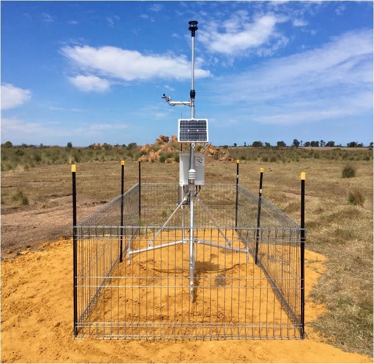
Station data are derived from weather stations that measure rainfall, temperature, wind and humidity or other observation platforms like flow gauges or soil moisture sensors. There are typically more rainfall stations than temperature stations.
Station data are in situ, point source data and representative of an immediate region, meaning they may not be representative of somewhere even 5km away. For example, in a flat area in the summer rainfall region temperature might be representative of a wide area but the nature of convective rainfall is such that it could be raining 5 km away from the measurement station but not at the station itself.
Station data may have temporal resolutions of minutes to days. Temperatures are usually reported as minimum, maximum and average daily temperature, rainfall is usually accumulated into daily rainfall and humidity is usually a daily averaged figure. Wind speeds can be reported hourly depending on the data source.
Data from stations are typically in an ascii format and easily imported into spreadsheets.
Although station data are measured and therefore apparently trustworthy, many errors creep into the data as a result of how they are collected, design of the measurement sensors and other factors.
Therefore station data must be quality controlled before use.
1.2 Gridded Data
In a gridded dataset, the grid cells have a particular horizontal grid resolution, i.e. the size of the grid, and the grid resolution may be coarse, e.g. 50 km, or fine, e.g. 1km. In each grid cell a single value for a particular variable, e.g. temperature or rainfall is provided. In course resolution data this means local modification of variables by e.g. topography or vegetation at the sub-grid scale cannot be captured and the value of the variable is presented as representative of the entire area covered by the grid.
Gridded observation datasets are generated in a number of ways. They can be simple interpolations between station data such as the widely used CRU (Climate Research Unit) data set. They may be satellite derived data such as the CMORPH (CPC MORPHing technique): High resolution precipitation (60S-60N) and TRMM: Tropical Rainfall Measuring Mission data set; or a blend of satellite and station data such as the CHIRPS: Climate Hazards InfraRed Precipitation with Station data (version 2) and GPCP (Daily): Global Precipitation Climatology Project data; or satellite, station and reanalysis data e.g. the Global high-resolution precipitation: MSWEP dataset.
Gridded data products do not necessarily have the same spatial and temporal resolutions. These vary between 2.5 x 2.5 degrees at a monthly time scale (GPCP: Monthly) to sub-daily time step at 0.1 degrees (10km) (MSWEP).
1.3 Reanalysis Data
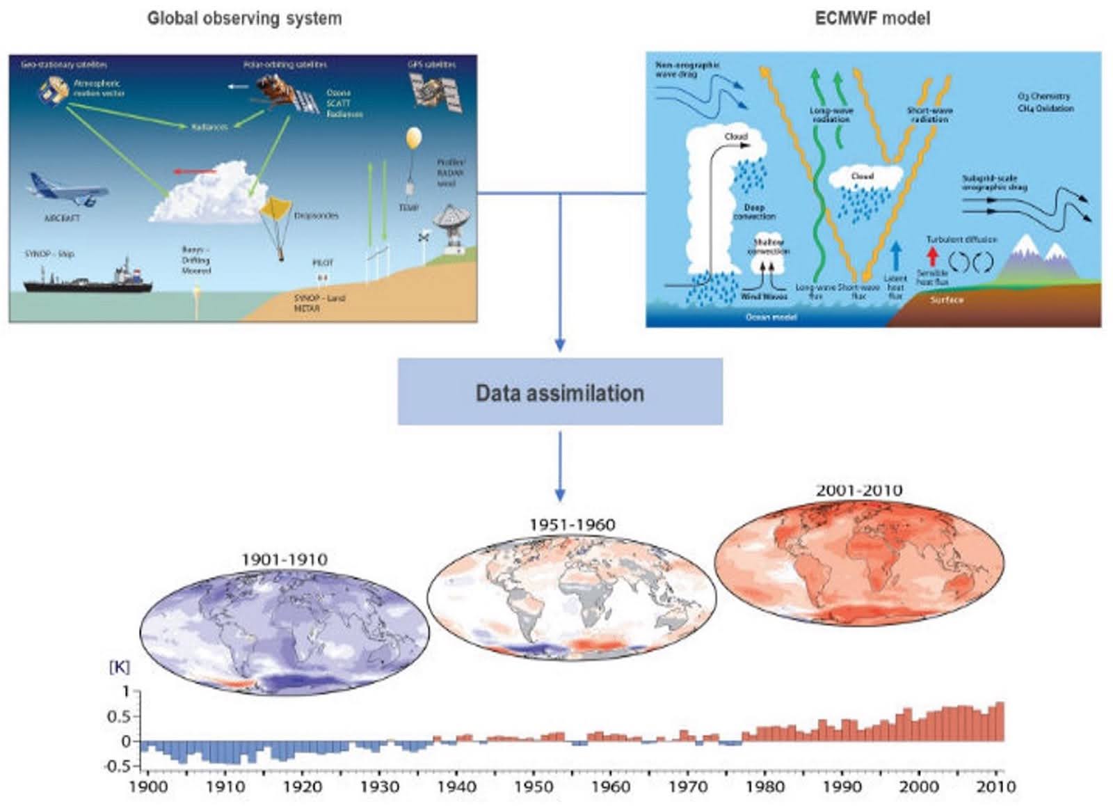
Climate reanalysis data refers to a dataset that combines weather observations with modern climate models to recreate past atmospheric conditions. Unlike raw observational data, reanalysis provides a complete and consistent record of the atmosphere, land surface, and oceans over an extended period. This is achieved by assimilating a variety of data sources, including satellite observations, weather station data, and other environmental measurements, into a climate model that then produces data at a global scale typically every three or one hour.
Different climate reanalysis products have different spatial and temporal resolutions and provided data for different periods, e.g. the latest product from the European Centre for Medium-Range Weather Forecasts (ECMWF) is the ERA-5 reanalysis that has data at an hourly time step, at a spatial resolution of 31km from January 1940 to present whereas the original reanalysys, the National Centre for Environmental Prediction (NCEP-NCAR) reanalysis has a 6-hourly timestep, a spatial resolution of 2.5 degrees and is available from January 1948 to December 2022.
Reanalysis data are typically provided globally in a netCDF or GRIB format, which requires processing to extract for a particular location.
1.4 Data formats
Ascii
Data in ascii or csv format are text-based data often used in spreadsheets for analysis. Climate data in this format are often from weather stations (see section on Weather Station data).
Binary format (NetCDF and GRIB)
Most climate data from global and regional climate models, including reanalysis data, is not in ascii format but in a binary format. The two most common of these are NetCDF and GRIB formats. These formats facilitate storage of the large volumes of data that climate models produce.
On some data download sites, e.g. the Copernicus Climate Data Store (CDS), it is possible to specify and extract a region or grid cell using latitude-longitude coordinates. Although the data have to be downloaded in NetCDF or GRIB formats there is software that can convert these data to ascii format including CDO (climate data operators), python (read in and convert the netcdf file to a dataframe then write the dataframe to ascii using df.to_csv), R (by converting the netcdf file to raster and then to ascii). Or submit the file to ChatGPT which will convert to ascii.
2. Seasonal forecast data
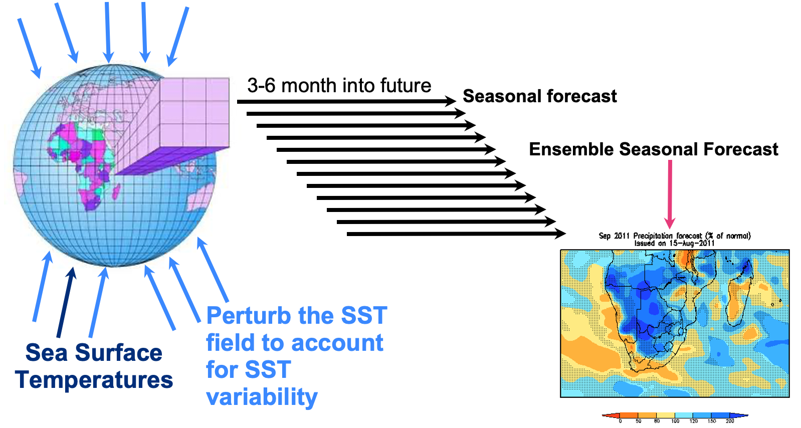
A seasonal forecast predicts the climate conditions over a period of one to six months and provides an overview of the likely climate conditions for the upcoming season. They are typically presented as how different conditions are predicted to be compared to a long-term mean ( the “normal”) and structured probabilistically, e.g.” There is a 60% chance that rainfall will be below normal in the next season, a 30 % chance it will be normal and a 10% change it will be above normal. There is a 90% chance temperatures will be above normal and a 10% chance they will be normal.”
Seasonal forecasts are produced by global climate models and in one seasonal forecast between 10 and up to 50 simulations are run for the season, this is termed a “10 (or 50)-member ensemble”. Each ensemble member is started a few hours later than the previous ensemble member; in a small ensemble (e.g. 10 members) this lag may be a day.
Running multiple member ensembles allows the forecast to span a wide probability space as
which provide many variables however temperature and precipitation anomalies are most often presented in forecasts.
Seasonal forecast data can be downloaded from several sources including the Copernicus Climate Data Store (https://climate.copernicus.eu/seasonal-forecasts). See Case study 2 below.
3. Multi-year forecasts - Decadal Prediction
Beyond the seasonal scale are multi-year to decadal predictions. Decadal forecasts provide information about the next 5-10 years and are dependent on predictions of the state of the ocean and how the oceanic circulation will evolve over the next few years and its subsequent impact on the atmosphere.
Decadal forecasts provide information about natural variability in the climate system and how it might evolve in the next few years in the context of a globally warming world. Decadal forecasting has, potentially, an important role to play here in assessing the probability of extremes in the next few years, and can be used for long-term planning and potentially facilitate the adaptation of different sectors to climate variability and change.
The World Meteorological Organization (WMO) releases a Global Annual to Decadal Climate Update each year (https://library.wmo.int/records/item/68910-wmo-global-annual-to-decadal-climate-update) and the forecasts are available from https://decadal.bsc.es/forecast.
4. Climate Change Data
Climate change data is primarily sourced from the World Climate Research Programme’s Coupled Model Intercomparison Project (CMIP), which provides a comprehensive framework for climate modeling and analysis. CMIP brings together climate models from research institutions worldwide, allowing for standardized comparisons and assessments of future climate projections. These climate models simulate the Earth’s climate system by incorporating various physical, chemical, and biological processes, generating data on temperature trends, precipitation patterns, sea level changes, and more. The models run simulations based on different greenhouse gas emission scenarios, known as Shared Socioeconomic Pathways (SSPs) or Representative Concentration Pathways (RCPs), which reflect varying levels of future human activity and policy decisions. By comparing these scenarios, scientists can assess a range of potential climate outcomes, from aggressive mitigation efforts to high-emission trajectories, helping to inform strategies for climate adaptation and mitigation.
B. Climate Models
Climate models are complex computer simulations that try to replicate the Earth’s climate system by representing the interactions between the atmosphere, oceans, land surface, and ice. They are based on fundamental physical principles, such as the laws of thermodynamics and fluid dynamics, and use mathematical equations to describe processes like radiation, convection, and cloud formation. To accurately simulate climate conditions, these models are “forced” at their boundaries with external inputs, such as observed or projected sea surface temperatures, greenhouse gas concentrations, volcanic activity, and solar radiation. Sea surface temperatures influence atmospheric circulation patterns and moisture availability, while greenhouse gases affect the planet’s energy balance by trapping heat in the atmosphere. By adjusting these boundary conditions, climate models can simulate both historical climate trends and predict future changes under different environmental scenarios.
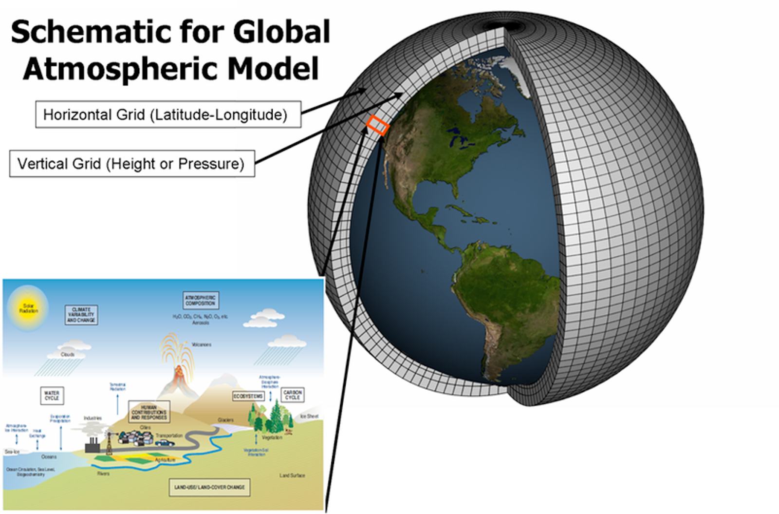
Climate models divide the Earth into a three-dimensional grid, with each grid cell representing a specific area of the atmosphere or ocean; the size of these cells determines the model’s spatial resolution. The average spatial resolution of CMIP6 global climate models typically ranges from 100 to 250 kilometers for atmospheric variables, meaning one value for e.g. rainfall is provided for a large spatial area and is not representative of the local scale. Impact models including malaria models usually require fine scale, high spatial resolution data, so using low resolution climate model data is likely to produce questionable results.
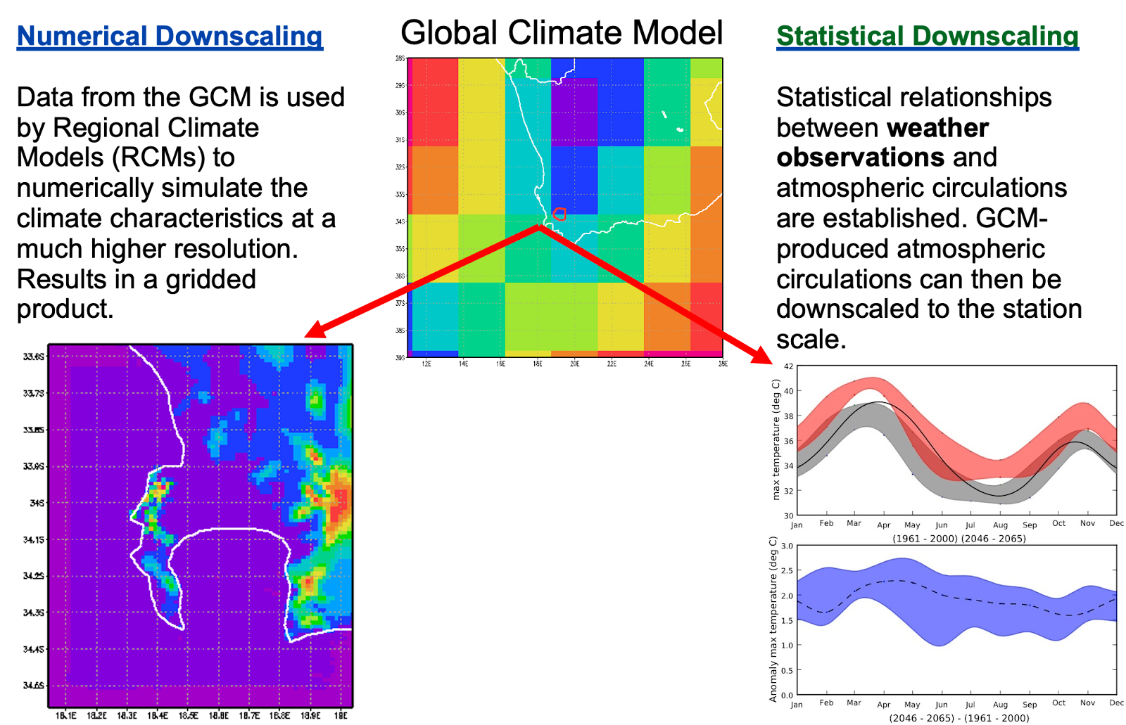
Higher-resolution models can capture finer-scale climate features, such as regional weather patterns and extreme events, but require significantly more computational power. Coarse resolution data can also be downscaled to finer resolutions by regional climate models (numerical downscaling) or through statistical methods. These data are more appropriate for use in impact models, however, the data should be bias corrected before being used for reasons described below.
C. Bias Correction
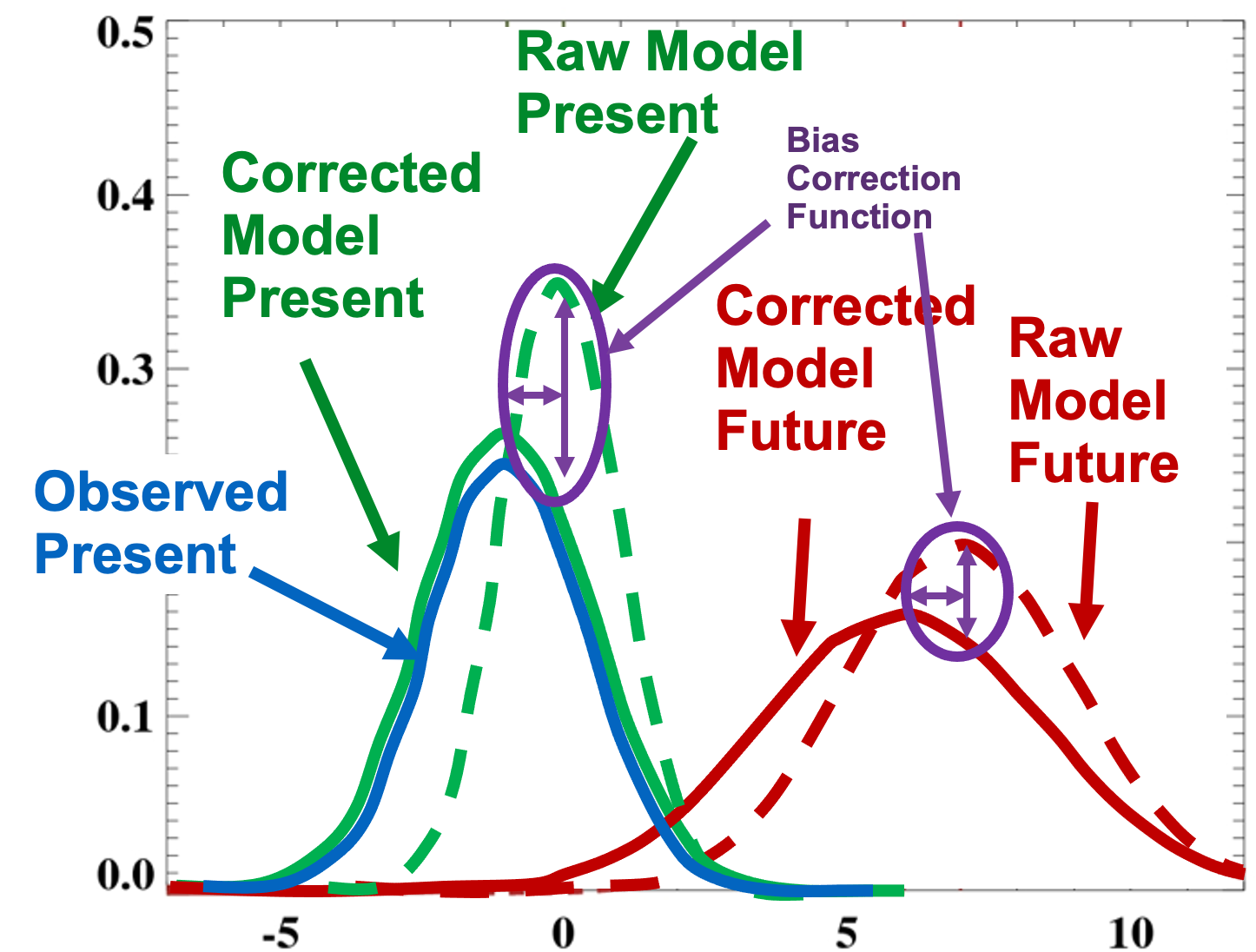
Bias correction of climate data involves adjusting climate model outputs to better match observed data, reducing systematic discrepancies between the model’s predictions and actual measurements. This process is crucial for improving the accuracy and reliability of climate model data that will be used by downstream impact models including malaria models.
Climate data used by impact models must be biased corrected before the impact model is run.
Many bias correction methods exist but most follow a procedure that adjusts the mean and variability of the climate model data towards the observed.
See Bias correction presentation
D. Climate Data Resources
Climate data is sourced from a variety of institutions and programs that provide comprehensive datasets for research and policy analysis. An excellent resource in understanding the different available data is the Climate Data Guide. This site gives an overview of almost all available climate data sources and provides download links.
One of the primary sources of climate model data is the World Climate Research Programme’s Coupled Model Intercomparison Project (CMIP), which offers climate model outputs from global research centers (CMIP6 Data). Observational climate data is provided by organizations like the National Oceanic and Atmospheric Administration (NOAA), which offers extensive historical records on temperature, precipitation, and atmospheric conditions NOAA Climate Data. The Copernicus Climate Data Store provides reanalysis datasets like ERA5, which combine historical observations with model data to create detailed global climate records ECMWF ERA5. Additionally, the Intergovernmental Panel on Climate Change (IPCC) hosts a data distribution center that provides access to climate scenarios, observational data, and model outputs used in their assessment reports IPCC Data Distribution Centre. One further resource is the Climate Information Portal, developed by the Swedish Meteorological and Hydrological Institute on behalf of the World Meteorological Organization (WMO) and World Climate Research Programme (WCRP). These resources are essential for understanding past, present, and future climate conditions.
E. Case Studies
1. Download the ERA5 climate reanalysis data for a study malaria in southern Africa
Data required
- Reanalysis data to use in a malaria modeling study, variables required are daily rainfall accumulated rainfall and daily mean temperature.
- Reanalysis data to use in a malaria modeling study, variables required are daily rainfall accumulated rainfall and daily mean temperature.
- Optional: Observation data if required to verify the reanalysis data if appropriate
Where to get the data
- The Copernicus Climate Change Service (CCS) data store ERA5 Reanalysis single level page
Navigate to the ERA5 reanalysis data page of the Copernicus Climate Data Store website.
- Register on the CDS if not yet registered
- Read the Overview Tab to understand the data and if more information if desired read documents on the Documentation Tab.
On the Download page select the following:
- Product - Select Reanalysis
- Variables - we suggest selecting and downloading 1 variable at a time to avoid delays in the download time. Large download requests are computationally costly and receive a lower priority. It’s advised to create smaller requests instead. The CDS can execute multiple download requests at a time so several smaller requests are better than single large requests.
- Time period - years, months or seasons and days can be selected depending on the study.
- Set the sub-region of interest - the default is to download the global dataset but it is possible to extract a sub-region (or single grid point). This sub-regions is set on the data portal.
- Submit the request - once submitted it is possible to monitor progress of your request
- Download the data when it becomes available and name the file appropriately.
The data are in NetCDF format and need to be post processed in order to be used in the malaria model. Reanalysis data may be bias corrected if enough observation data is available but most often is used as is in the impact model.
2. Download climate data to assess the next malaria season
Data required
- Daily rainfall, temperature and wind data for the coming season are available from several data sources.
- Data are also available from previous seasons and may be evaluated for skill against observations.
Where to get the data
- We suggest the Copernicus Climate Change Service Climate Data Store (CDS) as it is relatively easy to use. To get to the seasonal forecast data either search for “Seasonal forecast daily and subdaily data on single levels” or go to this link:
https://cds.climate.copernicus.eu/datasets/seasonal-original-single-levels?tab=overview
At least 5 lead time hours should be selected to span the range of probability, we suggest 1 every 24 hours i.e. 0, 24, 48, 72, 120, 144. A domain or single grid cell can be selected using latitude-longitude coordinates.