About the data
ERA5 is the fifth-generation reanalysis dataset produced by ECMWF (European Centre for Medium-Range Weather Forecasts), providing a detailed, global view of the climate. Covering the period from 1940 to near real-time, ERA5 combines vast amounts of historical observations with modern weather forecasting models, ensuring a globally complete, physically consistent record. The gridded dataset is available at a high spatial resolution of 0.25° (approximately 28 km by 28 km at the equator, varying slightly by latitude) and offers data at hourly intervals, providing sub-daily time resolution. It includes a wide range of surface and upper-air variables, supporting a broad spectrum of applications and research fields.
ERA5 is continuously updated, with data typically available within about one week of real time. Regular updates and corrections ensure the quality and completeness of the dataset over time.
ECMWF has made several subsets of the ERA5 reanalysis dataset available to meet different user needs. These include distinctions between data provided at pressure levels versus single levels (surface and near-surface variables), and at different temporal resolutions (hourly and monthly averages). For the purposes of this site, we focus on the “ERA5 hourly data on single levels from 1940 to present” subset, which offers high-resolution, near-surface climate variables suitable for a wide range of applications.
For more information regarding ERA5 datasets see ERA5-Dataset Documentation.
Users can also find more information about the ERA5 dataset here:
Climate Data Store: ERA5 hourly data on single levels from 1940 to present
Climate Data Guide: ERA5 atmospheric reanalysis
Summary
| Name | ERA5 (hourly data on single levels from 1940 to present) |
| Institution | ECMWF |
| Product type | reanalysis |
| Domain | global |
| Resolution | 0.25° x 0.25° |
| Period | 1940 - near real-time |
| Frequencies | hourly |
| Variables | precipitation, temperature, others |
| Update frequency (latency) | daily (+-5 days) |
Variables
| Variable Name | Variable Description | Units |
|---|---|---|
| 2m temperature | temperature of air at 2m above the surface of land, sea or inland waters | kelvin |
| Total precipitation | accumulated liquid and frozen water, comprising rain and snow, that falls to the Earth’s surface | meters |
| 10m u-component of wind | horizontal speed of air moving towards the east, at a height of ten meters above the surface of the Earth | meters per second |
| 10m v-component of wind | horizontal speed of air moving towards the north, at a height of ten meters above the surface of the Earth | meters per second |
For a comprehensive list of variables, you can refer to the dataset’s documentation on the Copernicus Climate Data Store.
Accessing the data
ERA5 is a widely used reanalysis dataset and can be downloaded from several different platforms. We focus here on the ERA5 hourly data on single levels from 1940 to present subset.
The ERA5 dataset is provided by the European Centre for Medium-Range Weather Forecasts (ECMWF) through the Copernicus Climate Change Service (C3S), with the Climate Data Store serving as the primary access point for ERA5 data. Users can download data directly from the ERA5 hourly data on single levels from 1940 to present dataset page. The CDS provides a user-friendly interface for selecting variables, spatial and temporal ranges, and output formats. Data is available in both GRIB and NetCDF formats.
Guidance on how to download ERA5 data via the Climate Data Store is available here
| Version | Variables | Resolution | Spatial Extent | File Format |
|---|---|---|---|---|
| Latest (updated daily) | 2m temperature, Total precipitation, 10m u-component of wind, 10m v-component of wind, 2m dewpoint temperature etc. A comprehensive list is available on the CDS dataset page. | 0.25° (~28km x ~28km) | Global/User specified | GRIB (.grib), NetCDF (.nc) |
The KNMI Climate Explorer provides access to ERA5 data with tools for analysis and visualization. The dataset can be specified on their Daily Select a field page. The ERA5 data available through KNMI is at daily resolution, with an ‘Africa’ subset included. Users can extract data for specific locations or regions and perform statistical analyses directly on the platform. Data provided in NetCDF format.
| Version | Variables | Resolution | Spatial Extent | File Format |
|---|---|---|---|---|
| Typically up-to-date | A selection of variables including temperature, precipitation, and wind. | 0.25° (~28km x ~28km), 0.5° (~55.5km x ~55.5km) | User specified | netCDF (.nc) |
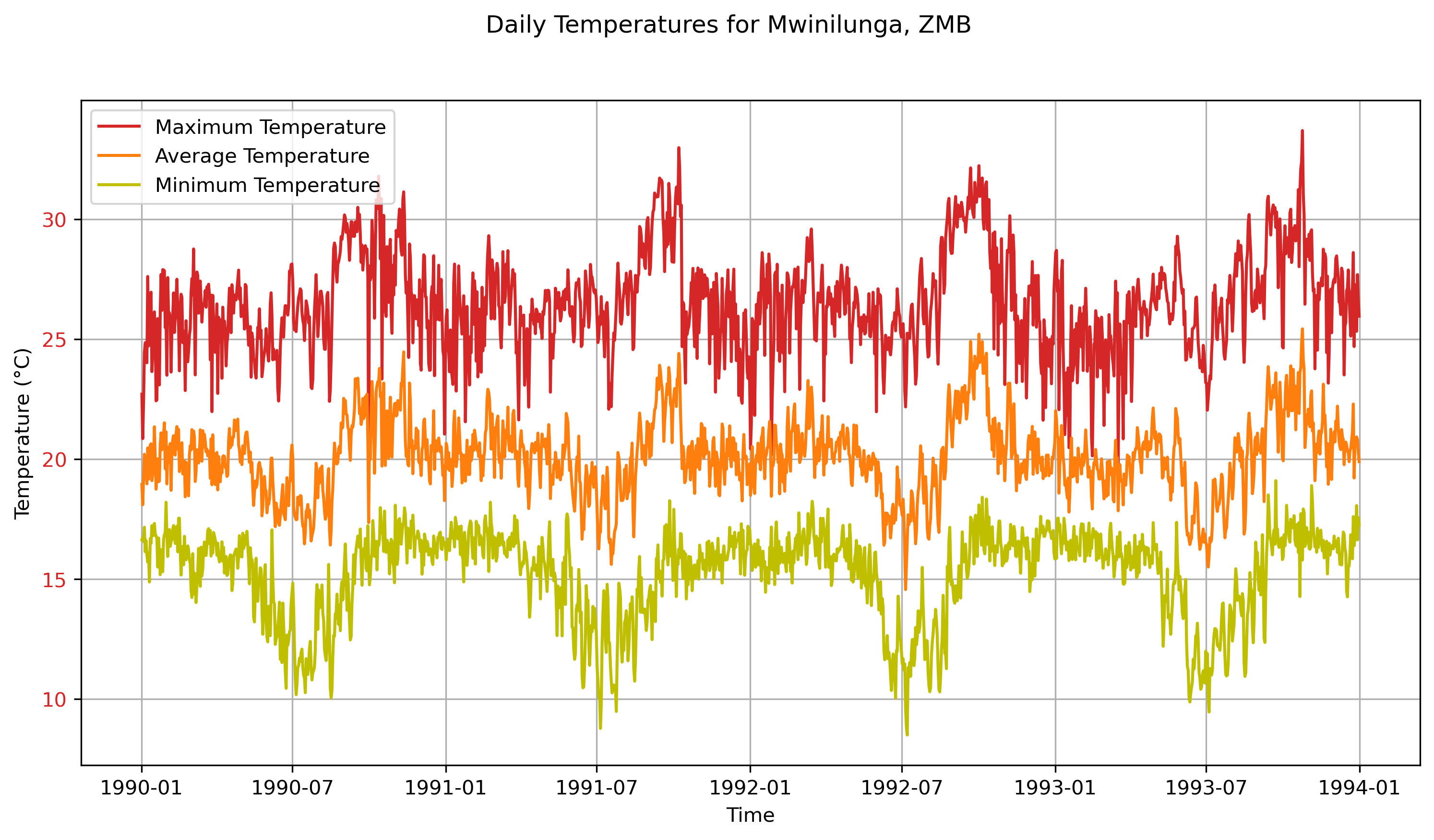
What the data looks likes
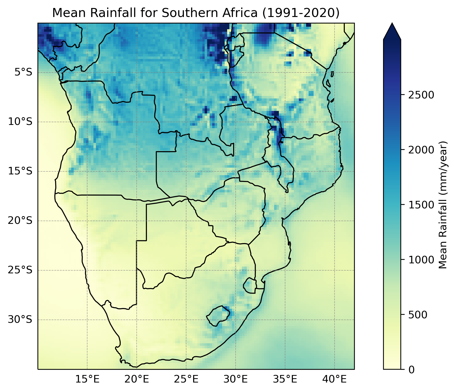
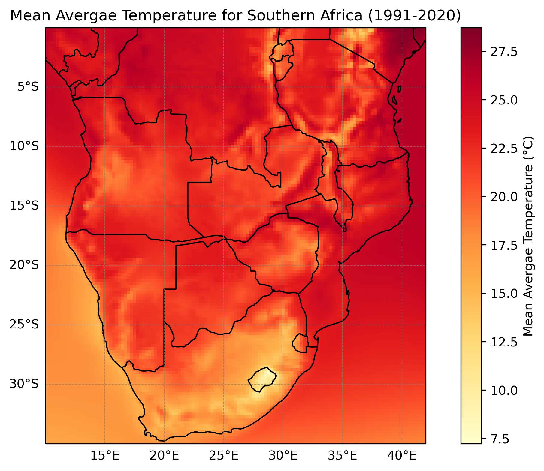
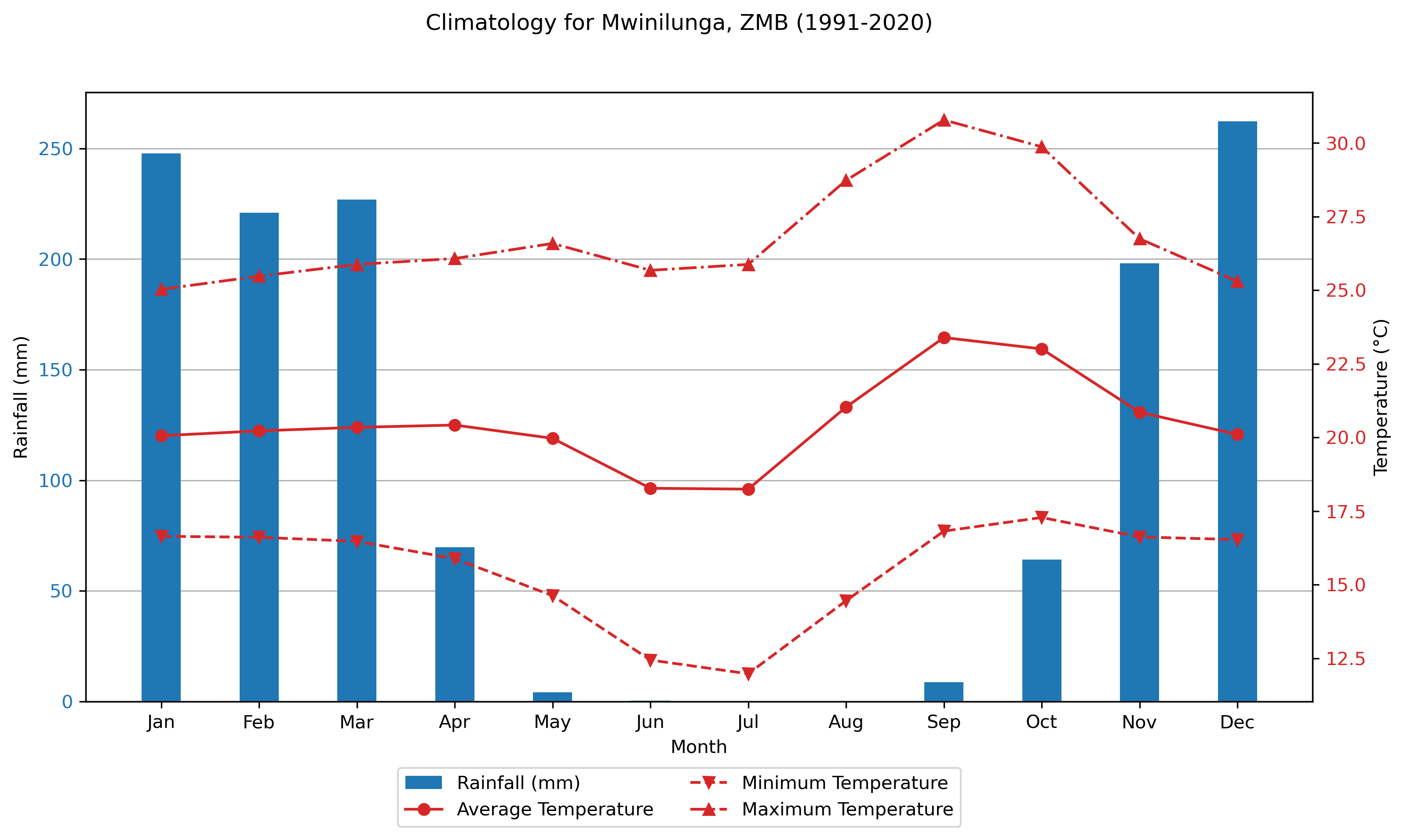
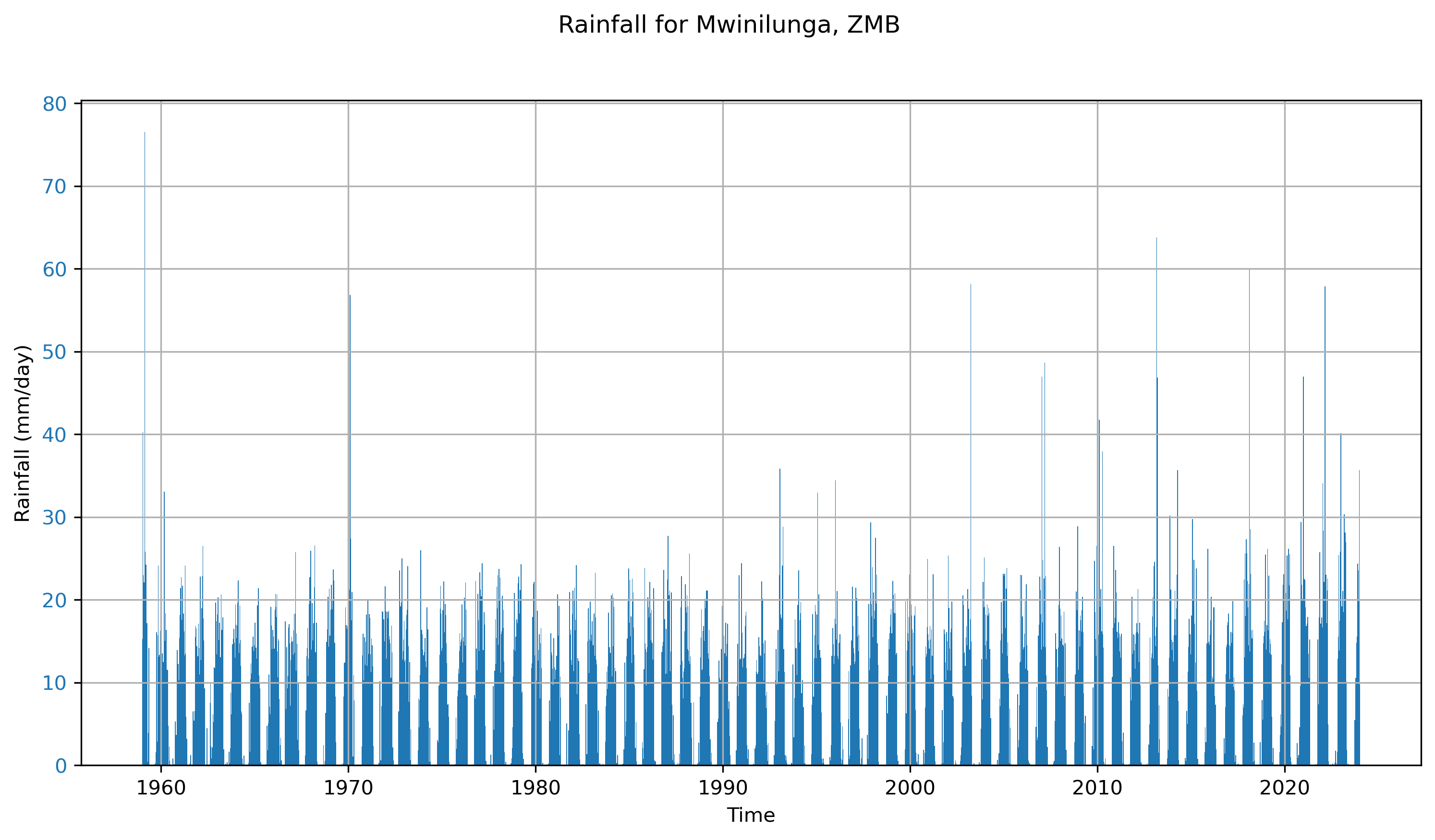
Below are a few plots to give a better sense of what the ERA5 dataset looks like. The first two are spatial plots over Southern Africa, illustrating the spatial resolution and the coarseness of the 0.25° × 0.25° grid. The final three plots focus on a single grid cell and show the seasonal cycle and time series data for that location.
Key points to consider
ERA5 is a global reanalysis dataset produced by combining model output with a wide range of historical observations using data assimilation techniques. It reflects a blend of satellite, in situ, aircraft, and other observational sources, integrated using the ECMWF Integrated Forecast System (IFS). Through this system, vast amounts of observations are brought together into a consistent model framework, resulting in a physically coherent dataset suitable for climate monitoring and research.
The quality and density of observations vary across space and time, particularly in earlier decades and over data-sparse regions. ERA5 provides uncertainty estimates for many variables through ensemble-based statistics, such as the standard deviation from the 10-member ensemble. These can be used as proxies to assess confidence in the data at specific times and locations.
ERA5 data is available at hourly resolution and can be aggregated to daily or monthly time scales. The dataset includes many surface and atmospheric variables, and its sub-daily time resolution supports detailed temporal analysis. It also enables the derivation of additional variables, such as relative humidity, from core fields like air temperature and dew point temperature. The reanalysis is updated daily with only a few days’ delay, making it suitable for near-real-time analysis. As a model-observation hybrid, ERA5 offers spatially and temporally complete outputs, which can be particularly valuable in regions or periods with limited direct observations.
Users should be aware that the skill of ERA5 data varies by variable, due to how the dataset is produced. ERA5 is derived from a global climate model with fixed spatial resolution, meaning it represents the Earth using a grid. As a result, it can struggle to accurately capture small-scale (‘sub-grid’) processes, such as localized convective rainfall (e.g. thunderstorms). Consequently, rainfall data tends to be less skillful, especially in regions dominated by convective processes or with sparse observational coverage. Temperature data, on the other hand, generally has higher skill, as it is strongly constrained by assimilated observations and tends to be more spatially consistent than rainfall. Comparing ERA5 data with local observations is recommended to assess its reliability.
Specific variables in ERA5 are defined and derived in distinct ways:
The temperature variable ‘2m temperature’ in ERA5 represents the air temperature at two meters above the surface. Over land, near-surface temperature observations from weather stations are combined with the model output to improve accuracy. However, ERA5 does not explicitly represent urban environments, so it may not fully capture the ‘urban heat island’ effect often observed in cities. Environmental factors such as land type and vegetation also influence the 2 meter temperature. Over the ocean, the 2 meter temperature is strongly influenced by sea surface temperatures (SST), which are derived from a combination of satellite observations (since 1982) and in-situ measurements (prior to 1982).
The precipitation variable ‘total precipitation’ in ERA5 includes all forms of precipitation (e.g. rain, snow, sleet, and hail). Unlike temperature, precipitation observations are not directly used to adjust the model so the data reflects the model’s best estimate based on its representation of physical processes. However, ERA5’s precipitation is influenced by other observations, such as satellite measurements of humidity in the atmosphere. ERA5 precipitation estimates rely heavily on parameterizations (simplified equations) to represent small-scale (‘sub-grid’) processes like thunderstorms, which can reduce accuracy in certain regions.
The wind vector variables ‘10m u-component’ and ‘10m v-component’ in ERA5 represent the U (east-west) and V (north-south) wind components 10 meters above the surface. These variables are not directly predicted by the model and are calculated from the model’s surface and atmospheric conditions outputs. Observational data is combined with the model outputs to provide the best estimate of near-surface wind conditions.
Strengths
- Provides a consistent, physically-based reconstruction of weather and climate over time.
- Offers hourly data since 1940, allowing analysis at high temporal resolution.
- Covers a wide range of variables, useful for many climate-health applications, including malaria modelling.
- Includes ensemble-based uncertainty estimates for many parameters.
Limitations
- The accuracy of ERA5 depends on the quality and availability of assimilated observations, which are limited in some regions and periods (especially before the satellite era or over data-sparse regions like parts of Africa).
- It is not an observational dataset but a model–observation hybrid; as such, it may smooth or misrepresent localized extremes or fine-scale variability.
- Can be complex and data-intensive to work with.
Citing the data
Hersbach, H., Bell, B., Berrisford, P., Biavati, G., Horányi, A., Muñoz Sabater, J., Nicolas, J., Peubey, C., Radu, R., Rozum, I., Schepers, D., Simmons, A., Soci, C., Dee, D., Thépaut, J-N. (2023): ERA5 hourly data on single levels from 1940 to present. Copernicus Climate Change Service (C3S) Climate Data Store (CDS), DOI: 10.24381/cds.adbb2d47 (Accessed on DD-MMM-YYYY)
Terms of use
All users of data uploaded on the Climate Data Store (CDS) must:
- provide clear and visible attribution to the Copernicus programme by referencing the web catalogue entry
- acknowledge according to the data licence
- cite each product used
For guidance on acknowledging or citing the Climate Data Store, see this page. For an example of how to cite ERA5 data specifically, refer to this ERA5 use case.
How to plot this data?
In this example, we demonstrate how to visualise ERA5 data using the ERA Explorer application provided by Climate Data Store (CDS). The ERA Explorer application allows users to explore the historical climate for anywhere on earth using the ERA5 reanalysis dataset and focuses on four key variables, temperature, rainfall, wind and humidity, all of which are important for Malaria modelling. In the below example we will focus on two different locations in southern Africa.
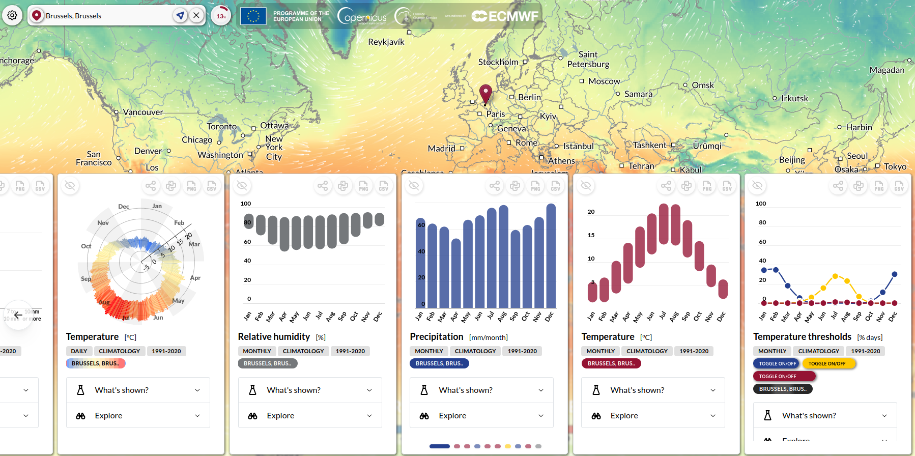
Users can select a location of interest by clicking on the global interactive map. The application then calculates a set of climate statistics for the selected grid cell (0.25° x 0.25° resolution), which are displayed as a series of plots. These plots can be downloaded as PNG images, and the underlying data can be downloaded in CSV format. The site also links to example Python notebooks to help users understand, replicate, or customize the code.
Note: The data represents average conditions for the entire grid cell, not the precise local environment. A guidance section, accessible via the “?” icon, provides information on how to use the app; the organisation, the ERA5 dataset and about the data, and how to interpret the plots presented in the app.
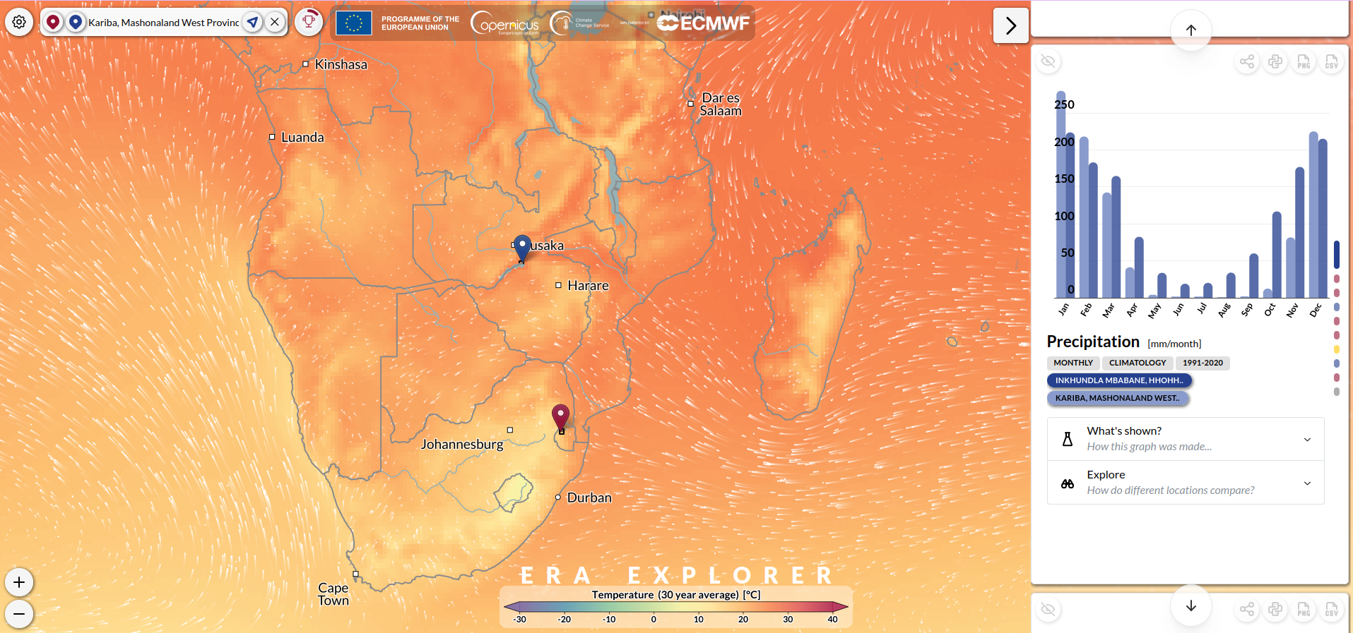
To illustrate, two locations in southern Africa with contrasting climates were selected (Fig. 3):
- Kariba, Zimbabwe
- Mbabane, Eswatini
The ERA Explorer provides several types of visualisations which include:
- Monthly climatologies (temperature, rainfall and relative humidity)
- Annual timeseries (temperature and rainfall)
- Annual anomalies (temperature)
- Daily climatologies (temperature)
- Hourly climatologies (wind)
Each plot is generated automatically, with a brief explanation below describing the method used. While most plots look straightforward, some involve complex processing—particularly those showing relative humidity or hourly wind climatologies.
If users wish to generate their own plots, it is recommended to download the data from the application and to refer to the example python notebooks provided.
Monthly Climatologies
![Monthly temperature climatology for Kariba (Zimbabwe) and Mbabane (Eswatini) for the period 1991-2020. We can see Kariba is consistently warmer than Mbabane throughout the year. Kariba’s temperatures peak in spring (Sept–Nov), while Mbabane experiences its warmest temperatures in summer (Dec–Feb). Both locations have their coolest periods in winter (Jun–Aug). Source: Copernicus Climate Change Service (C3S). (2025). ERA Explorer [Web application]. Retrieved from https://era-explorer.climate.copernicus.eu/](images/Temperature_monthly_climatology_26.30S31.17E_16.52S28.80E.png)
![Monthly precipitation climatology for Kariba (Zimbabwe) and Mbabane (Eswatini) for the period 1991-2020. Both locations experience a distinct wet season from November to March, with Kariba generally receiving more rainfall during the early summer months (Dec–Feb). Kariba has an extended dry season from May to October, while Mbabane tends to receive more consistent rainfall throughout its drier season. Source: Copernicus Climate Change Service (C3S). (2025). ERA Explorer [Web application]. Retrieved from https://era-explorer.climate.copernicus.eu/](images/Precip_monthly_climatology_26.30S31.17E_16.52S28.80E.png)
![Monthly precipitation climatology for Kariba (Zimbabwe) and Mbabane (Eswatini) for the period 1991-2020. Mbabane generally exhibits higher relative humidity than Kariba throughout the year. While both locations experience lower humidity during the dry season, Kariba shows a more pronounced drop during the hot, dry months of early spring (Sept–Oct), whereas Mbabane’s lowest levels occur during the cooler winter months (Jun–Aug).Source: Copernicus Climate Change Service (C3S). (2025). ERA Explorer [Web application]. Retrieved from https://era-explorer.climate.copernicus.eu/](images/Humidity_monthly_climatology_26.30S31.17E_16.52S28.80E.png)
Annual Timeseries
![Annual average temperature for Kariba (Zimbabwe) and Mbabane (Eswatini) for the period 1940-2024. Kariba is consistently around 8°C warmer than Mbabane. A clear warming trend is evident in both locations. Source: Copernicus Climate Change Service (C3S). (2025). ERA Explorer [Web application]. Retrieved from https://era-explorer.climate.copernicus.eu/](images/Temperature_annual_timeseries_26.30S31.17E_16.52S28.80E.png)
![Annual total precipitation for Kariba (Zimbabwe) and Mbabane (Eswatini) for the period 1940-2024. Mbabane consistently receives more annual rainfall than Kariba, with both locations showing high interannual variability. Source: Copernicus Climate Change Service (C3S). (2025). ERA Explorer [Web application]. Retrieved from https://era-explorer.climate.copernicus.eu/](images/Precip_annual_timeseries_26.30S31.17E_16.52S28.80E.png)
Daily Climatologies
![Daily temperature climatology for Kariba (Zimbabwe) for the period 1991-2020. There are distinct cool and warm periods throughout the year. The hottest days and nights occur in late October to early November, while the coldest are observed in early July. Source: Copernicus Climate Change Service (C3S). (2025). ERA Explorer [Web application]. Retrieved from https://era-explorer.climate.copernicus.eu/](images/Temperature_daily_climatology_16.52S28.80E.png)
![Daily temperature climatology for Mbabane (Eswatini) for the period 1991-2020. The coldest days and nights occur in early July, while the warmest temperatures are more broadly distributed across the summer months (Dec–Feb), rather than peaking in a single period. Source: Copernicus Climate Change Service (C3S). (2025). ERA Explorer [Web application]. Retrieved from https://era-explorer.climate.copernicus.eu/](images/Temperature_daily_climatology_26.30S31.17E.png)
Hourly Climatologies
![Hourly climatological wind rose for Kariba (Zimbabwe) for the period 1991-2020. Wind direction is highly unidirectional with very little variation, indicating a dominant prevailing wind. The wind speed does vary, suggesting changes in intensity even though the direction remains relatively consistent. Source: Copernicus Climate Change Service (C3S). (2025). ERA Explorer [Web application]. Retrieved from https://era-explorer.climate.copernicus.eu/](images/Wind_annual_climatology_16.52S28.80E.png)
![Hourly climatological wind rose for Mbabane (Eswatini) for the period 1991-2020. The wind rose indicates that winds come from multiple directions, with a few directions (Westly, West Noth-Westly and South-Eastly) more common than others. This suggests a moderately variable wind regime without a single dominant direction. Wind speeds also show a wide range of variability. Source: Copernicus Climate Change Service (C3S). (2025). ERA Explorer [Web application]. Retrieved from https://era-explorer.climate.copernicus.eu/](images/Wind_annual_climatology_26.30S31.17E.png)
Annual Anomalies
![Climate warming stripes (annual temperature anomalies relative to the 1961–2010 reference period) for Kariba (Zimbabwe) and Mbabane (Eswatini) for 1940–2024. A clear concentration of red shades in recent decades highlights a warming trend at both locations. Source: Copernicus Climate Change Service (C3S). (2025). ERA Explorer [Web application]. Retrieved from https://era-explorer.climate.copernicus.eu/](images/Temperature_warming_stripes_26.30S31.17E_16.52S28.80E.png)
How can this data be used in disease modelling?
In endemic countries with year-round transmission, malaria cases still peak during the rainy season (November to April for most southern African countries). During this time, temperature and rainfall conditions favour vector development, thereby increasing the total mosquito population. A few specific malaria variables have been experimentally shown to be temperature-sensitive (Shapiro 2017; Suh 2024):
- The parasite extrinsic incubation period
- Vector gonotrophic cycle
- Human biting rate
- Daily survival/death rate of larval and adult vectors
- The egg to adult development rate
The egg to adult development rate is also rainfall-sensitive, as is oviposition and the carrying capacity of the environment.
Preparing the data
Using the CRU TS dataset, we obtain specific values for temperature over time, and model the historic impact of climatology on the vector population and subsequent incidence. We use mean air temperature as a proxy for surface temperatures.
There are different approaches to explicitly include environmental conditions into an infectious disease model. For this example, we use three equations from Traore (2017) and Agusto (2015; 2020) defining the effect of climate on the dynamics of malaria transmission. Specifically, the example below describes temperature-dependent human biting rate and mosquito mortality, as well as rainfall-dependent environmental carrying capacity.
Show the code
# Load the data
temperature_values <- bind_rows(
  read_csv("data/tas_daily_ERA5_19800101-20231231_Kariba.csv") |>
    mutate(City = "Kariba"),
  read_csv("data/tas_daily_ERA5_19800101-20231231_Mbabane.csv") |>
    mutate(City = "Mbabane")) |>
  select(time, tas, City) |>
  group_by(City) |>
  mutate(tas = case_when(
     as_date(time) == ymd("2018-06-29") ~ mean(c(tas[as_date(time) == ymd("2018-06-28")], tas[as_date(time) == ymd("2018-07-01")])),
    as_date(time) == ymd("2018-06-30") ~ mean(c(tas[as_date(time) == ymd("2018-06-28")], tas[as_date(time) == ymd("2018-07-01")])),
    TRUE ~ tas))  |> # fix outliers in 2018 due to artefact
  filter(time >= ymd("2014-01-01") & time <= ymd("2023-12-31") # start date of data

)

ggplot() +
  geom_point(data = temperature_values, aes(x = time, y = tas, colour = City)) +
  theme_health_radar() +
  scale_colour_manual_health_radar() +
  labs(
    title = str_wrap("Daily Mean Surface Air Temperature values in Kariba and Mbabane from 2014 to 2023", width = 50),
    x = "Year",
    y = "Temperature values (Celsius °)",
    caption = str_wrap("Changes in temperature over time. Kariba has higher temperatures on average, which may impact vector competence, depending on the primary Anopheles vector in the area and its behavioural habits. Source: tas daily ERA5")
  ) +
  ylim(0, NA)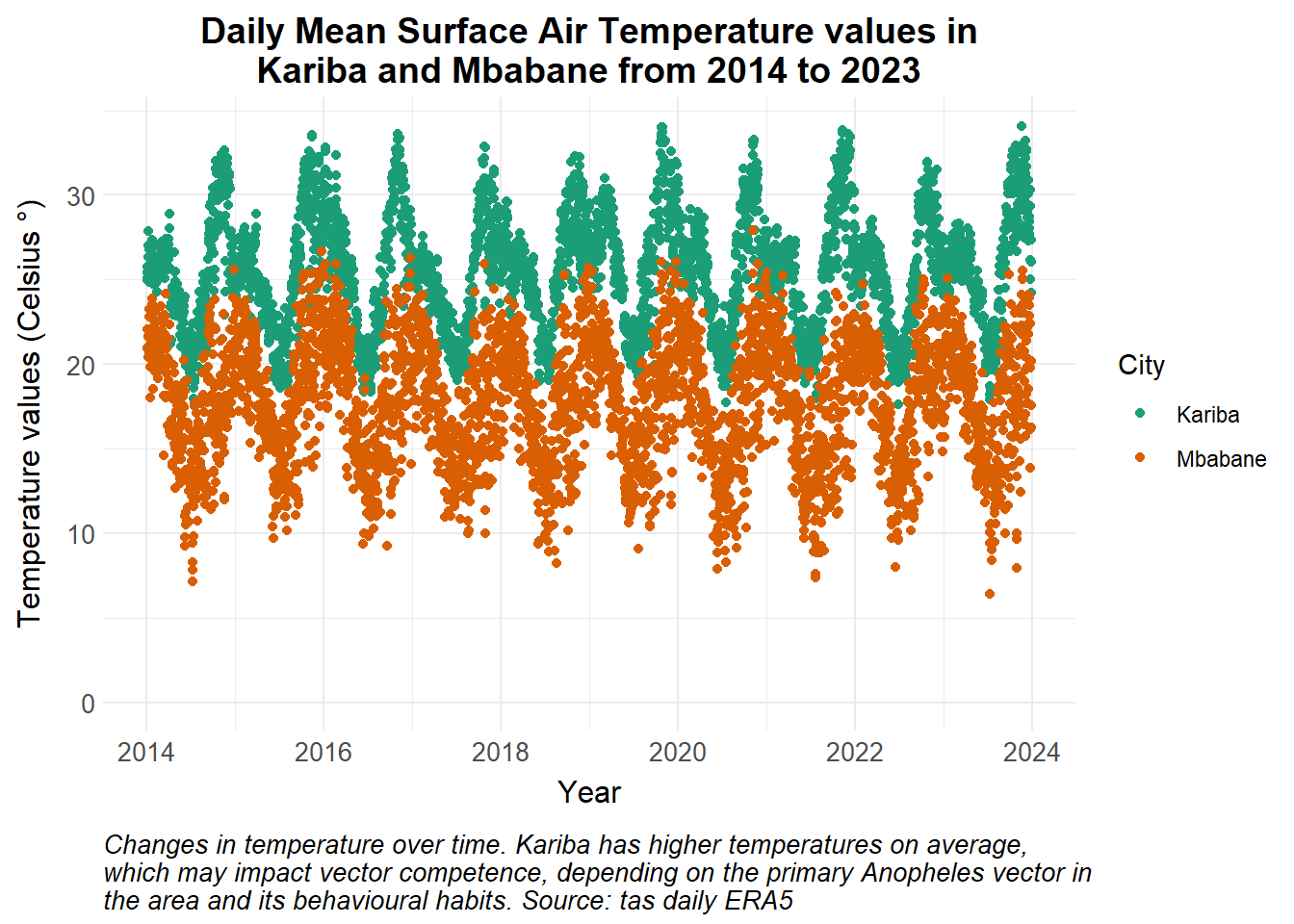
Show the code
# Load the data
rainfall_values <- bind_rows( read_csv("data/PRCPTOT_daily_ERA5_19800101-20231231_Kariba.csv") |>
mutate(City = "Kariba"),
read_csv("data/PRCPTOT_daily_ERA5_19800101-20231231_Mbabane.csv") |>
mutate(City = "Mbabane")) |>
select(time, pr, City) |>
filter(time >= ymd("2014-01-01") & time <= ymd("2023-12-31") # start date of data
)
ggplot() +
geom_point(data = rainfall_values, aes(x = time, y = pr, colour = City)) +
scale_colour_manual_health_radar() +
theme_health_radar() +
labs(
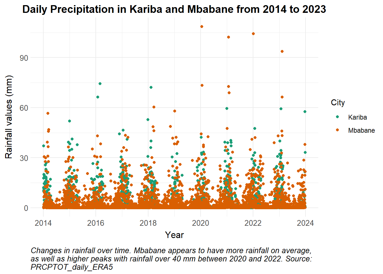
title = "Daily Precipitation in Kariba and Mbabane from 2014 to 2023",
x = "Year",
y = "Rainfall values (mm)",
caption = str_wrap("Changes in rainfall over time. Mbabane appears to have more rainfall on average, as well as higher peaks with rainfall over 40 mm between 2020 and 2022. Source: PRCPTOT_daily_ERA5")
) 
We incorporate these values into the mathematical model. Note that other models may include other variables such as altitude and humidity. For this example we will explore the mosquito populations and incidence in both cities, as influenced by the environmental conditions. We achieve this by assuming the same parameters and starting conditions in both cities, and only varying the inputs for rainfall and temperature.
Show the code
# Time points for the simulation
Y = 10 # Years of simulation
times <- seq(0, 365*Y, by = 1)

# Rainfall values for each city
rains_kariba <- (filter(rainfall_values, City == "Kariba"))$pr
rains_mbabane <- (filter(rainfall_values, City == "Mbabane"))$pr

# Temperature values for each city
temps_kariba <- (filter(temperature_values, City == "Kariba"))$tas
temps_mbabane <- (filter(temperature_values, City == "Mbabane"))$tas


# SEACR-SEI model
seacr <- function(times, start, parameters, rains_vec, temp_vec) {
  with(as.list(c(start, parameters)), {
    P = S + E + A + C + R + G
    M = Sm + Em + Im
    m = M / P

    t_day <- floor(times) + 1
    t_day <- pmin(t_day, length(rains_vec))  # prevent out-of-bounds

    rain <- rains_vec[t_day]
    temp <- temp_vec[t_day]

    # Temperature-dependent equations obtained from Traore 2017 and Agusto 2020
    # biting rate
    a <-  -0.00014*temp^2 + 0.027*temp - 0.322

    # daily oviposition rate
    ovi <- max(-0.153*temp^2 + 8.61*temp - 97.7, 0) # prevent values going below zero

    # death rate
    mu_m <- -log(-0.000828*temp^2 + 0.0367*temp + 0.522)

    # carrying capacity
    K <- max(Km*(rain+1), 1)  # ensure K stays above 1000

    # Force of infection
    Infectious = C + zeta_a*A #infectious reservoir
    lambda.v <- a*M/P*b*Im/M
    lambda.h <- a*c*Infectious/P

    # Differential equations/rate of change
    dSm = ovi*(1-M/K)*M - lambda.h*Sm - mu_m*Sm
    dEm = lambda.h*Sm - (gamma_m + mu_m)*Em
    dIm = gamma_m*Em - mu_m*Im

    dS = mu_h*P - lambda.v*S + rho*R - mu_h*S
    dE = lambda.v*S - (gamma_h + mu_h)*E
    dA = pa*gamma_h*E + pa*gamma_h*G - (delta + mu_h)*A
    dC = (1-pa)*gamma_h*E + (1-pa)*gamma_h*G - (r + mu_h)*C
    dR = delta*A + r*C - (lambda.v + rho + mu_h)*R
    dG = lambda.v*R - (gamma_h + mu_h)*G

    dCInc = lambda.v*(S+R)


    # Output
    list(c(dSm, dEm, dIm, dS, dE, dA, dC, dR, dG, dCInc))
  })
}


# Initial values for compartments (we use the same starting values for both cities here)

# Kariba, Zimbabwe
initial_state <- c(Sm = 50000, # susceptible mosquitoes
                   Em = 30000, # exposed and infected mosquitoes
                   Im = 10000, # infectious mosquitoes
                   S = 25000, # susceptible humans
                   E = 8000, # exposed and infected humans
                   A = 7000, # asymptomatic and infectious humans
                   C = 4000, # clinical and symptomatic humans
                   R = 5000, # recovered and semi-immune humans
                   G = 1000, # secondary-exposed and infected humans
                   CInc = 0 # cumulative incidence
)

# Country-specific parameters should be obtained from literature review and expert knowledge
parameters <- c(#a = 0.45, # human biting rate
                b = 0.5, # probability of transmission from mosquito to human
                c = 0.5, # probability of transmission from human to mosquito
                r = 1/21, # rate of loss of infectiousness after treatment
                rho = 1/160, # rate of loss of immunity after recovery
                delta = 1/150, # natural recovery rate
                zeta_a = 0.4, # relative infectiousness of of asymptomatic infections
                pa = 0.4, # probability of asymptomatic infection
                #mu_m = 1/10, # birth and death rate of mosquitoes
                mu_h = 1/(62*365), # birth and death rate of humans
                gamma_m = 1/10, # extrinsic incubation rate of parasite in mosquitoes
                gamma_h = 1/10, # extrinsic incubation rate of parasite in humans
                Km = 50000 # carrying capacity for mosquito egg laying and pupae and larval development
                )


# Run both models
outK <- ode(y = initial_state,
           times = times,
           func = seacr,
           parms = parameters,
           rains_vec = rains_kariba,
           temp_vec = temps_kariba)

outM <- ode(y = initial_state,
           times = times,
           func = seacr,
           parms = parameters,
           rains_vec = rains_mbabane,
           temp_vec = temps_mbabane)

# Post-processing model output into a dataframe

dfK <- as_tibble(as.data.frame(outK)) |>
  mutate(P = S + E + A + C + R + G,
         M = Sm + Em + Im,
         Inc = c(0, diff(CInc))) |>
  pivot_longer(cols = -time, names_to = "variable", values_to = "value") |>
  mutate(date = ymd("2014-01-01") + time,
         City = "Kariba")

dfM <- as_tibble(as.data.frame(outM)) |>
  mutate(P = S + E + A + C + R + G,
         M = Sm + Em + Im,
         Inc = c(0, diff(CInc))) |>
  pivot_longer(cols = -time, names_to = "variable", values_to = "value") |>
  mutate(date = ymd("2014-01-01") + time,
         City = "Mbabane")

df <- bind_rows(dfK, dfM) |>
  group_by(City)
Changes in vector population
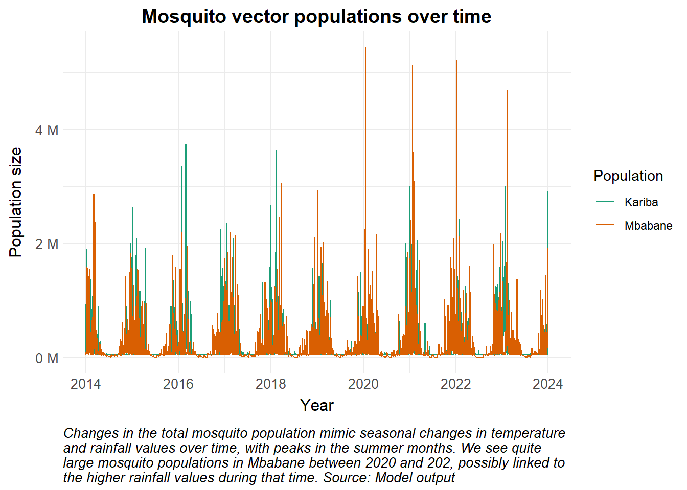
As mentioned earlier, environmental conditions affect the parasite and mosquito development, and as such we anticipate changes in the vector population to mimic the pattern in the temperature. In this example, we assume the human population stays constant as is shown in the panel on the right. The UN Population Data portal page describes human population growth in the context of disease modelling. In this example, we assume that the human population remains constant, and that humans can be exposed to and infected by an infectious mosquito while recovering from an initial infection (secondary infection).
Show the code
df |>
  filter(variable == "M") |>
  ggplot() +
  geom_line(aes(x = date, y = value, colour = City)) +
  theme_health_radar() +
  scale_colour_manual_health_radar() +
  scale_y_continuous(labels = scales::label_number(suffix = " M", scale = 1e-6)) +
  labs(
    title = "Mosquito vector populations over time",
    x = "Year",
    y = "Population size",
    colour = "Population",
    caption = str_wrap("Changes in the total mosquito population mimic seasonal changes in temperature and rainfall values over time, with peaks in the summer months. We see quite large mosquito populations in Mbabane between 2020 and 202, possibly linked to the higher rainfall values during that time. Source: Model output")
  )
Implications for transmission
The force of infection (i.e. the rate at which susceptible individuals become infected per unit time) is largely driven by the human biting rate, the ratio of vectors relative to hosts, the probability of transmission and the size of the infectious reservoir. Below, we see how the temperature has driven the rate of new cases through the temperature-dependent variables.
This is especially insightful when the model includes periods of time impacted by severe environmental conditions such as drought or flooding, and the consequences on malaria transmission dynamics are reflected in the incidence values. Note that the example below is not an actual reflection of malaria transmission in Kariba or Mbabane, and is merely illustrative. We plot the modelled clinical cases for the years 2014 to 2023, however, in reality the value of reported clinical cases may be smaller due to limitations in treatment access, availability of rapid diagnostic tests, and even test sensitivity.
Show the code
df |>
  filter(variable == "C", time > 100) |>
  ggplot()+
  geom_line(aes(x = date, y = value, colour = City)) +
  theme_health_radar() +
  scale_colour_manual_health_radar() +
  labs(
    title = "Daily symptomatic cases values in the human population",
    x = "Year",
    y = "Number of cases",
    caption = str_wrap("There are more cases during the summer months, where environmental conditions are suitable for mosquito breeding and malaria transmission. In Mbabane, case numbers rise sharply in the wet season and drop to near zero in the dry season, indicating a high seasonal amplitude. Kariba, however, displays sustained transmission throughout the year (even during winter), leading to a higher overall case burden annually. Source: Model output.")
  ) +
  ylim(0, NA)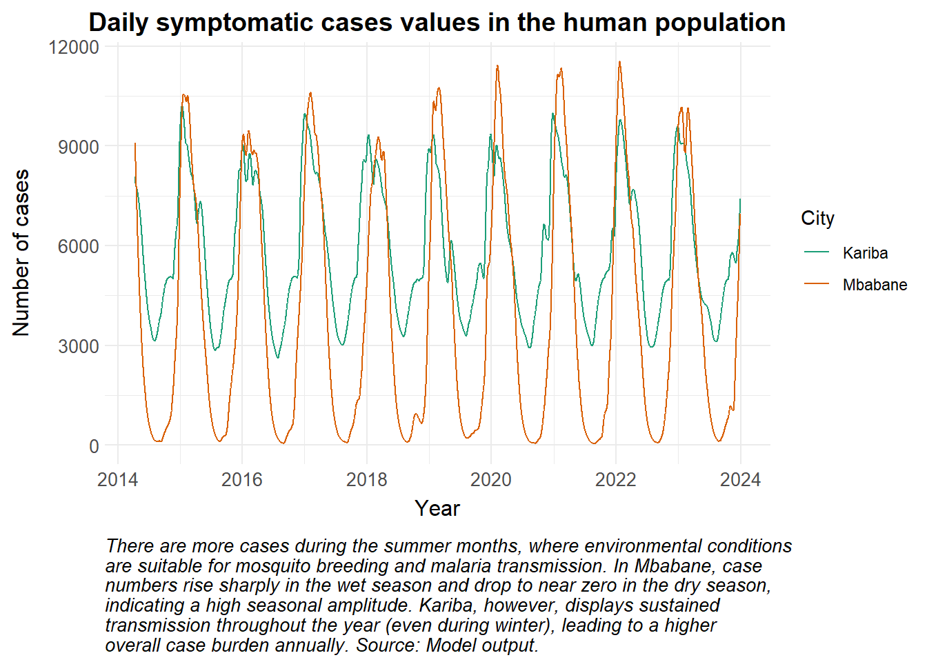
Policy implications
Models that incorporate temperature and rainfall explicitly may be used to forecast seasonal or year-to-year transmission patterns. This can be used to enable early warning systems for malaria outbreaks, as well as for temporal planning of interventions such as indoor residual spraying (IRS) for maximum impact. This approach also promotes multidisciplinary collaboration for policymakers across health, environmental, and climate sciences.
Citations
- Agusto F. B., Gumel A. B., & Parham P. E. Qualitative assessment of the role of temperature variations on malaria transmission dynamics. Journal of Biological Systems, 23(04), 1550030 (2015). https://doi.org/10.1142/S0218339015500308
- Agusto F.B. Optimal control and temperature variations of malaria transmission dynamics. Complexity, 1, 5056432 (2020). https://doi.org/10.1155/2020/5056432
- Traoré B., Sangaré B., Traoré S. A mathematical model of malaria transmission with structured vector population and seasonality. Journal of Applied Mathematics, 1, 6754097 (2017). https://doi.org/10.1155/2017/6754097
- Shapiro L.L.M., Whitehead S.A., & Thomas M.B. Quantifying the effects of temperature on mosquito and parasite traits that determine the transmission potential of human malaria. PLoS Biology 15(10), e2003489 (2017). https://doi.org/10.1371/journal.pbio.2003489
- Suh, E., Stopard, I.J., Lambert, B. et al. Estimating the effects of temperature on transmission of the human malaria parasite, Plasmodium falciparum. Nature Communications 15, 3230 (2024). https://doi.org/10.1038/s41467-024-47265-w